
Examples & Templates#
Copy-pasteable boilerplate code for common Malet workflows.
Minimal Experiment Setup#
End-to-end: define a YAML config and run experiments over a hyperparameter grid.
exp_config.yaml:
model: ResNet18
dataset: cifar10
num_epochs: 50
batch_size: 128

grid:
    seed: [1, 2, 3]
    lr: [0.001, 0.01, 0.1]
    optimizer: [sgd, adam]
train.py:
from functools import partial
from malet.experiment import Experiment

def train(config):
    # Your training logic here
    # ...
    return {'train_loss': [...], 'val_accuracy': [...]}

experiment = Experiment(
    './experiments/resnet_cifar10',
    partial(train),
    ['train_loss', 'val_accuracy'],
)
experiment.run()
Basic Plot Generation#
Common malet-plot invocations:
# Line plot of validation accuracy over epochs, one line per optimizer
malet-plot -exp_folder ./experiments/resnet_cifar10 \
    -mode curve-epoch-val_accuracy \
    -multi_line_fields 'optimizer' \
    -best_at_max

# Bar chart comparing optimizers at the last epoch
malet-plot -exp_folder ./experiments/resnet_cifar10 \
    -mode bar-optimizer-val_accuracy \
    -filter 'step last' \
    -best_at_max

# Heatmap of lr vs. optimizer
malet-plot -exp_folder ./experiments/resnet_cifar10 \
    -mode heatmap-lr\ optimizer-val_accuracy \
    -filter 'step last' \
    -best_at_max
Custom Plot with Python API#
Use avgbest_df and ax_draw_curve for fine-grained control:
import matplotlib.pyplot as plt
from malet.experiment import ExperimentLog
from malet.plot_utils.data_processor import avgbest_df
from malet.plot_utils.plot_drawer import ax_draw_curve

log = ExperimentLog.from_tsv('./experiments/resnet_cifar10/log.tsv')
df = log.melt_and_explode_metric()

# Average over seeds, pick best lr
processed = avgbest_df(
    df, 'val_accuracy',
    avg_over='seed',
    best_over=('lr',),
    best_at_max=True,
)

fig, ax = plt.subplots()
ax_draw_curve(ax, processed, label='ResNet18')
ax.set_xlabel('Epoch')
ax.set_ylabel('Val Accuracy')
ax.legend()
fig.savefig('custom_plot.pdf')
Real-World Plotting Examples (CIFAR-10 ResNet20)#
The following examples use a real experiment log included in the repository (tests/fixtures/cifar10_resnet20_log.tsv). The experiment compares ADMM and SAFE optimizers with SAM gradients on CIFAR-10 with ResNet20, sweeping over sparsity, label noise, and SAM radius (ρ).
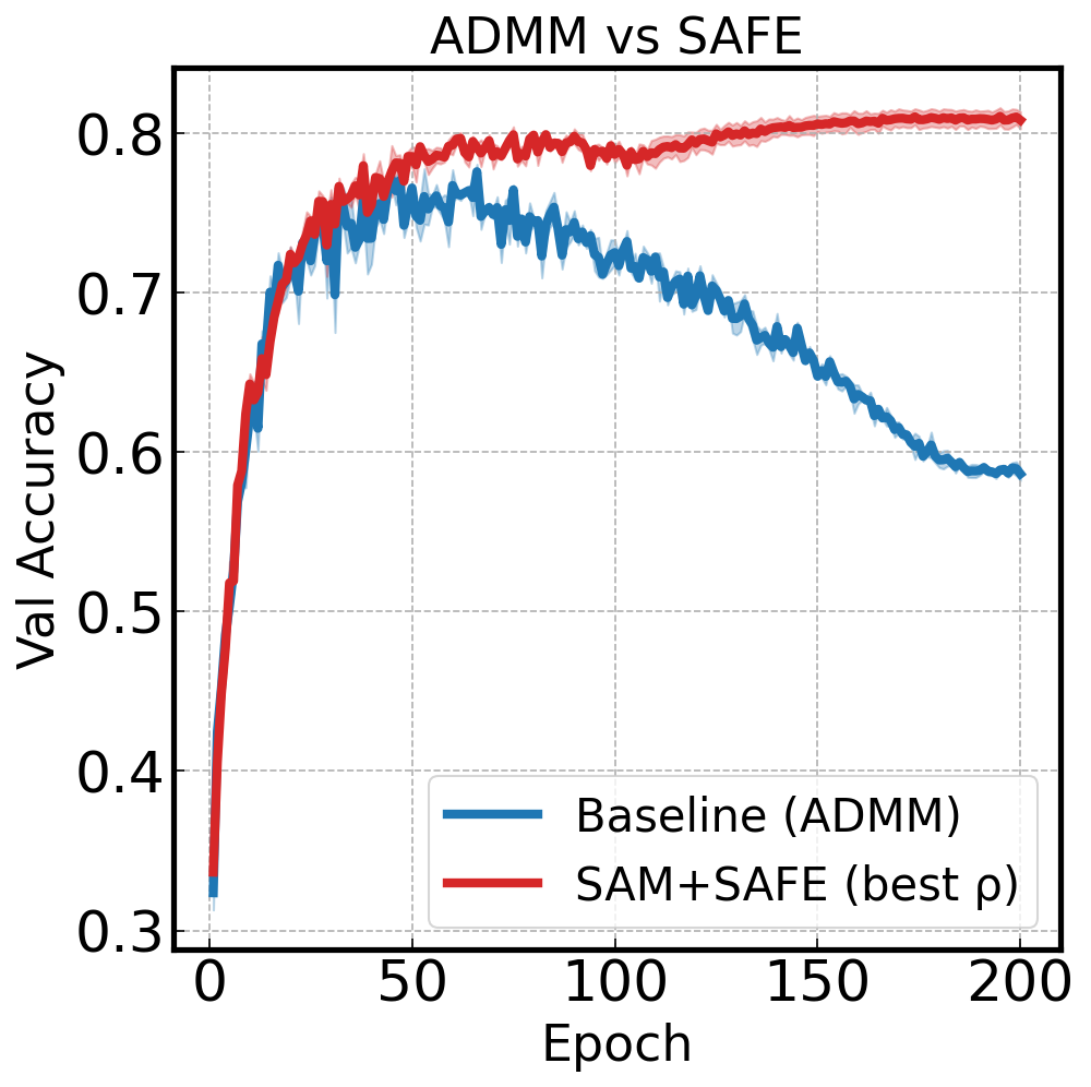
Compare Methods with Training Curves#
Plot baseline (ADMM) vs SAM+SAFE with shaded standard error across seeds:
import matplotlib.pyplot as plt
from malet.experiment import ExperimentLog
from malet.plot_utils.data_processor import avgbest_df, select_df
from malet.plot_utils.plot_drawer import ax_draw_curve

log = ExperimentLog.from_tsv('tests/fixtures/cifar10_resnet20_log.tsv')
df = log.melt_and_explode_metric()
df = select_df(df, {'metric': 'val_accuracy', 'noise': 0.5, 'sp': 0.9})

fig, ax = plt.subplots(figsize=(9, 6))

# Baseline: standard gradient + ADMM
base_df = select_df(df, {'grad_type': 'grad', 'optim': 'admm', 'rho': 0.0})
base_df = avgbest_df(base_df, 'metric_value', avg_over={'seed'}, best_at_max=True)
base_df = base_df.reset_index([n for n in base_df.index.names if n != 'step'], drop=True).sort_index()
ax_draw_curve(ax, base_df, label='Baseline (ADMM)', color='#1f77b4', annotate=False, std_plot='fill')

# SAM gradient + SAFE (best rho auto-selected)
sam_df = select_df(df, {'grad_type': 'sam_grad', 'optim': 'safe'})
sam_df = avgbest_df(sam_df, 'metric_value', avg_over={'seed'}, best_over={'rho'}, best_at_max=True)
sam_df = sam_df.reset_index([n for n in sam_df.index.names if n != 'step'], drop=True).sort_index()
ax_draw_curve(ax, sam_df, label='SAM+SAFE (best ρ)', color='#ff7f0e', annotate=False, std_plot='fill')

ax.set_xlabel('Epoch')
ax.set_ylabel('Val Accuracy')
ax.set_title('Baseline vs SAM+SAFE — CIFAR-10 ResNet20')
ax.legend()
ax.grid(True, linestyle='--', alpha=0.4)
fig.savefig('baseline_vs_sam.png', dpi=150, bbox_inches='tight')
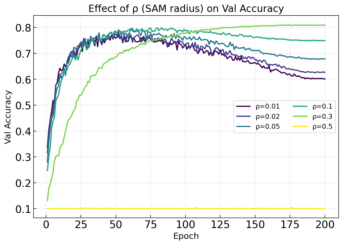
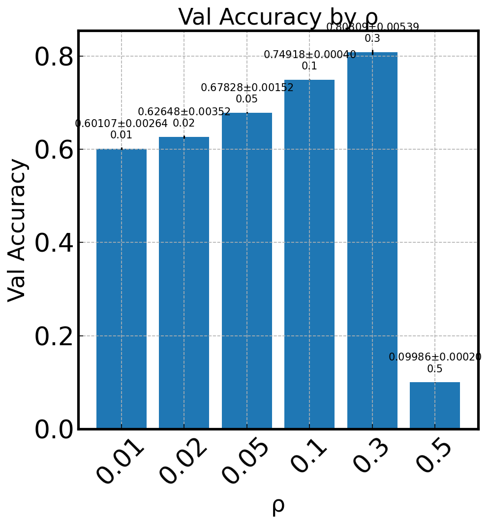
Hyperparameter Sweep Visualization#
See how different values of ρ (SAM perturbation radius) affect training:
fig, ax = plt.subplots(figsize=(9, 6))
df = log.melt_and_explode_metric()
df = select_df(df, {'metric': 'val_accuracy', 'noise': 0.5, 'sp': 0.9,
                     'optim': 'safe', 'grad_type': 'sam_grad'})

cmap = plt.cm.viridis
for i, rho in enumerate([0.01, 0.02, 0.05, 0.1, 0.3, 0.5]):
    p_df = select_df(df, {'rho': rho})
    p_df = avgbest_df(p_df, 'metric_value', avg_over={'seed'}, best_at_max=True)
    p_df = p_df.reset_index([n for n in p_df.index.names if n != 'step'], drop=True).sort_index()
    ax_draw_curve(ax, p_df, label=f'ρ={rho}', color=cmap(i/5),
                  annotate=False, std_plot='none', linewidth=2)

ax.set_xlabel('Epoch')
ax.set_ylabel('Val Accuracy')
ax.set_title('Effect of ρ (SAM radius) on Val Accuracy')
ax.legend(ncol=2)
ax.grid(True, linestyle='--', alpha=0.4)
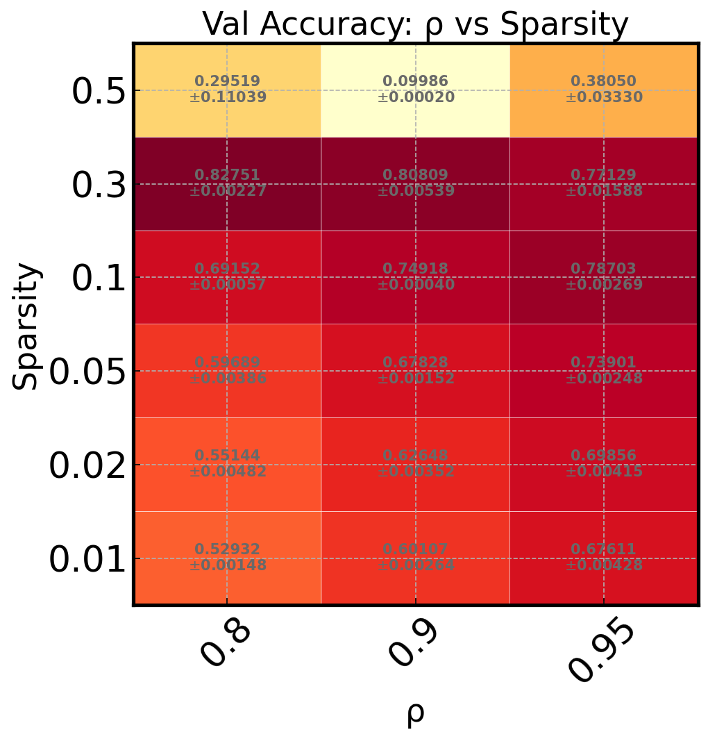
Heatmap of Two Hyperparameters#
Quickly identify optimal hyperparameter combinations:
from malet.plot_utils.plot_drawer import ax_draw_heatmap

df = log.melt_and_explode_metric(step=-1)
df = select_df(df, {'metric': 'val_accuracy', 'noise': 0.5,
                     'optim': 'safe', 'grad_type': 'sam_grad'})
df = avgbest_df(df, 'metric_value', avg_over={'seed'}, best_at_max=True)
# Keep only rho and sp as index levels
df = df.reset_index([n for n in df.index.names if n not in ('rho', 'sp')], drop=True).sort_index()

fig, ax = plt.subplots(figsize=(8, 5))
ax_draw_heatmap(ax, df, cmap='YlOrRd', annotate=True)
ax.set_xlabel('ρ (SAM radius)')
ax.set_ylabel('Sparsity')
ax.set_title('Val Accuracy: ρ vs Sparsity')
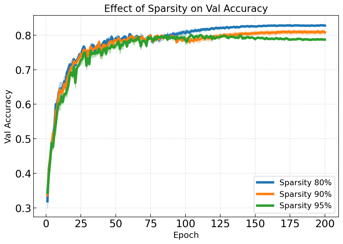
Comparing Sparsity Levels#
Show how pruning aggressiveness trades off with accuracy:
fig, ax = plt.subplots(figsize=(9, 6))
df = log.melt_and_explode_metric()
df = select_df(df, {'metric': 'val_accuracy', 'noise': 0.5,
                     'optim': 'safe', 'grad_type': 'sam_grad'})

colors = {0.8: '#1f77b4', 0.9: '#ff7f0e', 0.95: '#2ca02c'}
for sp in [0.8, 0.9, 0.95]:
    p_df = select_df(df, {'sp': sp})
    p_df = avgbest_df(p_df, 'metric_value', avg_over={'seed'},
                      best_over={'rho'}, best_at_max=True)
    p_df = p_df.reset_index([n for n in p_df.index.names if n != 'step'], drop=True).sort_index()
    ax_draw_curve(ax, p_df, label=f'Sparsity {int(sp*100)}%',
                  color=colors[sp], annotate=False, std_plot='fill')

ax.set_xlabel('Epoch')
ax.set_ylabel('Val Accuracy')
ax.set_title('Effect of Sparsity on Val Accuracy')
ax.legend()
ax.grid(True, linestyle='--', alpha=0.4)
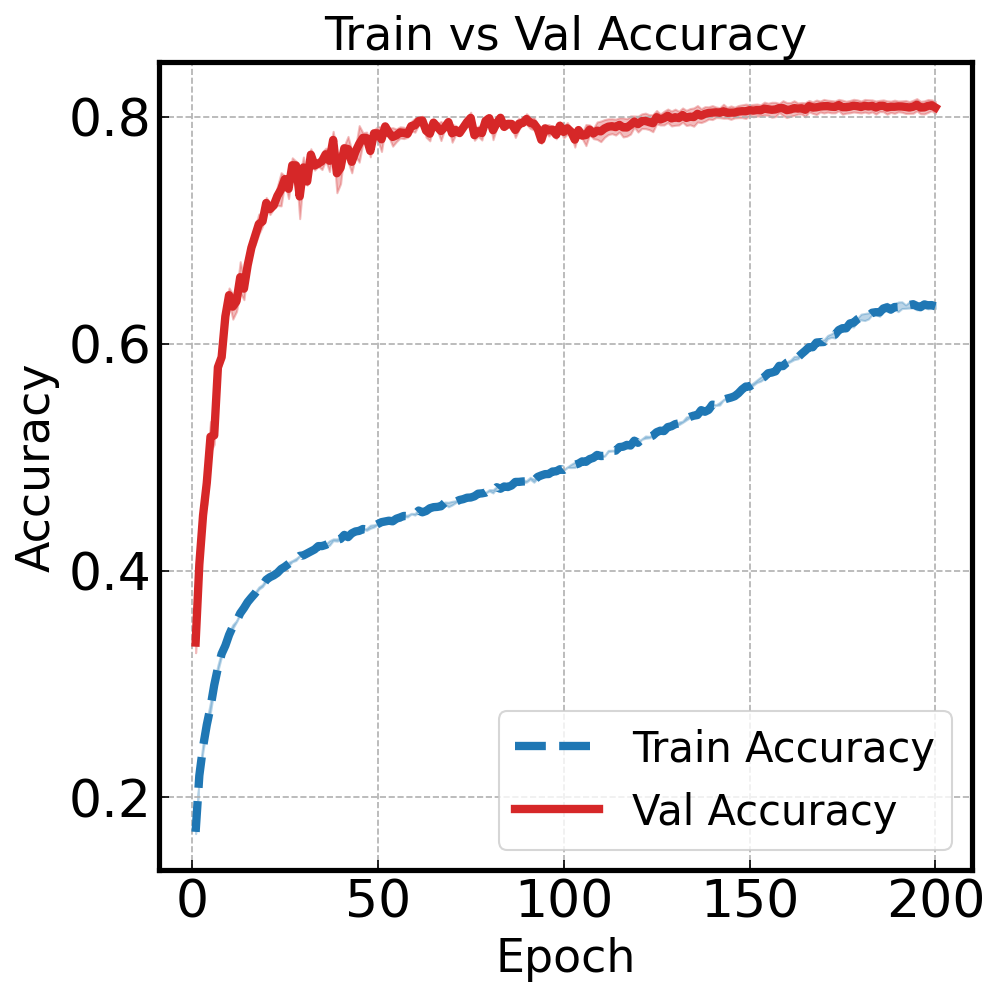
Train vs Val: Visualizing Generalization#
Overlay train and validation accuracy to spot overfitting:
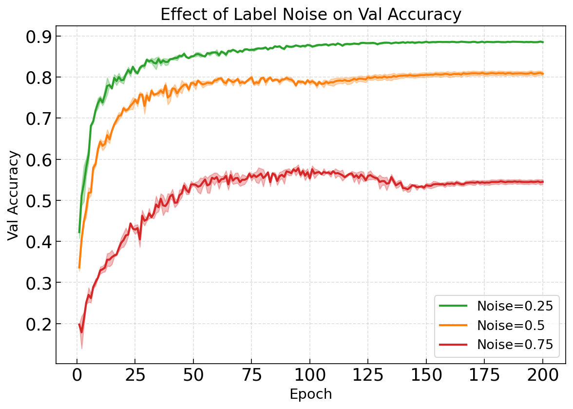
Robustness to Label Noise#
Compare performance degradation under increasing label corruption:
Bar Charts for Final Results#
Log Manipulation#
Loading, filtering, deriving fields, and inspecting logs:
from malet.experiment import ExperimentLog

# Load
log = ExperimentLog.from_tsv('log.tsv')
print(log.static_configs)
print(log.df)
print(log.grid_dict())

# Derive a new field
log.derive_field(
    'lr_group',
    lambda lr: 'high' if lr > 0.01 else 'low',
    'lr',
    is_index=True,
)

# Rename fields
log.rename_fields({'val_accuracy': 'val_acc'})

# Drop unused fields
log.drop_fields(['train_loss'])

# Check if a config exists and retrieve its metrics
config = {'seed': 1, 'lr': 0.01, 'optimizer': 'adam'}
if config in log:
    metrics = log[config]
    print(metrics)
Parallel GPU Training (Slurm)#
Slurm array job template with partitioning + queueing:
#!/bin/bash
#SBATCH --job-name=malet_train
#SBATCH --gres=gpu:1
#SBATCH --array=0-3

python train.py ./experiments/resnet_cifar10 \
    --total_splits=4 \
    --curr_split=$SLURM_ARRAY_TASK_ID \
    --filelock \
    --configs_save
After all jobs finish, merge the split logs:
from malet.experiment import Experiment

Experiment.resplit_logs('./experiments/resnet_cifar10', target_split=1)
W&B Sweep Integration#
Load sweep results from Weights & Biases and plot with Malet:
from malet.experiment import ExperimentLog

log = ExperimentLog.from_wandb_sweep(
    entity='my-team',
    project='my-project',
    sweep_ids=['abc123'],
    logs_file='./experiments/wandb_sweep/log.tsv',
    get_all_steps=True,
)
log.to_tsv()
# Plot directly
malet-plot -exp_folder ./experiments \
    -wandb_sweep_id 'my-team/my-project/abc123' \
    -mode curve-step-val_loss
Checkpoint & Resume#
Training with intermediate checkpoints for long-running jobs:
from functools import partial
from malet.experiment import Experiment

def train(config, experiment):
    metric_dict = {'train_loss': [], 'val_accuracy': []}

    # Resume from checkpoint if this config previously failed
    if config in experiment.log:
        metric_dict = experiment.get_metric_info(config)[0]

    start_epoch = len(metric_dict['train_loss'])
    for epoch in range(start_epoch, config.num_epochs):
        # ... training logic ...
        metric_dict['train_loss'].append(loss)
        metric_dict['val_accuracy'].append(acc)

        # Checkpoint every 10 epochs
        if (epoch + 1) % 10 == 0:
            experiment.update_log(config, **metric_dict)

    return metric_dict

experiment = Experiment(
    './experiments/long_run',
    partial(train),
    ['train_loss', 'val_accuracy'],
    checkpoint=True,
    filelock=True,
)
experiment.run()